XDS: CPOL
CPOL: C-Band Polarimetric Radar
General Data Description
The polarimetric radar is a scanning 5 cm wavelength radar that uses a 10 minute cycle that includes a volume scan, an RHI (Range Height Indicator) scan over the ARM Darwin site and a vertical “cloud mode” scan.
Measurement Description
The 10-minute 3D gridded product description: specific differential phase, and cross-correlation between the signals at two polarizations.
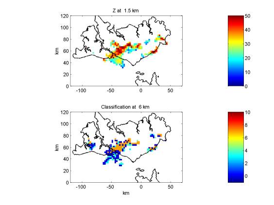
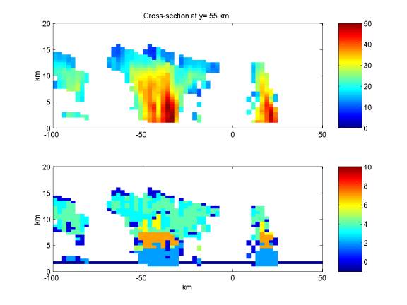
The reflectivity (in dBZ) is stored. The data are also combined and used to estimate/classify the microphysical type where there is significant echo (Keenan, 2003). The microphysical classes are:
| 0 | Unclassified |
| 1 | Drizzle |
| 2 | Rain |
| 3 | Dry low density snow |
| 4 | Dry high density snow |
| 5 | Melting snow |
| 6 | Dry graupel |
| 7 | Wet graupel |
| 8 | Small hail < 2 cms |
| 9 | Large hail > 2 cms |
| 10 | Rain hail mix |
These data are also archived. The data is stored as ascii for easy reading. The format of the ascii files is as follows:
1)  date(YYYYMMDD)  time(HHMM)
2)  radar latitude, radar longitude, Xmin,Xmax,number of xvalues, Ymin,Ymax,number of y values,Zmin,Zmax,number of zvalues
3)  for each z value
       {
             for each y value
             {
                  reflectivity, hydroclassification pairs for each x value
             }
      }
      reflectivity equals X when missing or no data
      hydroclassification equals x when missing or no precipitation.
      Therefore most of the time data is   ' X     x'.
The data for each 10 min volume is in a separate file. A program to read the other two types of files is available below under Data User Notes.
Rainfall units are given as millimeters/hour.
Temporal Coverage
The polarimetric radar (Keenan et al, 1998) is located at Gunn Point (12.2522S, 131.0428E), approximately 25 km to the NE of the ARCS3 site.
The data from the volume scan is interpolated onto a Cartesian grid with a horizontal resolution for the 3-D product of 2.5 km and a vertical resolution of 0.5 km over a domain +/- 150 km in the horizontal and from 0.5 to 20 km in altitude.
The 2-D rain products cover the same horizontal domain but with a resolution of 1.0 km.
Contacts
ARM Data Center
Data Source
Institution
Australian Bureau of Meteorology (BOM)
Data User Notes
A sample MATLAB code to read the 10 minute 3D gridded product files (1) above is:
fnam='c:\data\class_files\Dec02_02\cpol_hydroclass_20021202_0540.ASCII';
  fid = fopen(fnam)
  %fid = fopen('zhclass.txt','r');
  %
  cline1 = fscanf(fid,'%14c',1);
  adate = str2num(cline1(1,1:8))
  ahhmm = str2num(cline1(1,10:13))
  %
  cline2 = fscanf(fid,'%79c',1);
  slatr = str2num(cline2(1,1:8))
  slongr = str2num(cline2(1,10:18))
  xmin = str2num(cline2(1,20:26))
  xmax = str2num(cline2(1,28:34))
  nx = str2num(cline2(36:38))
  delx=(xmax-xmin)/(nx-1)
  ymin = str2num(cline2(1,40:46))
  ymax = str2num(cline2(1,48:54))
  ny = str2num(cline2(56:58))
  dely=(ymax-ymin)/(ny-1)
  zmin = str2num(cline2(1,60:66))
  zmax = str2num(cline2(1,68:74))
  nz = str2num(cline2(76:78))
  delz=(zmax-zmin)/(nz-1)
  %                       1       2       3      4        5       6       7      8        9      10      11      12      13      14
  vals =
  fscanf(fid,'%81c%*1c%81c%*1c%81c%*1c%81c%*1c%81c%*1c%81c%*1c%81c%*1c%81c%*1c%81c%*1c%81c%*1c%81c%*1c%81c%*1c%81c%*1c%36c%*1c',[1089,inf]);
  size(vals)
  aamzw = reshape(vals,9,585640);
  bbmzw = aamzw';
  czh = bbmzw(:,2:6);
  chclass = bbmzw(:,8:9);
  azhc = zeros(1,585640);
  ahclass = zeros(1,585640);
  %
  for i = 1:585640
     azhc(i) = -9999.;
     j = strcmp(czh(i,1:5),'  X  ');
     if j < 1
        azhc(i) = str2num(czh(i,1:5));
     end
     ahclass(i) = -1;
     k = strcmp(chclass(i,1:2),' x');
     if k < 1
         ahclass(i) = str2num(chclass(i,1:2));
     end
  end
  zh = reshape(azhc,121,121,40);
  hclass = reshape(ahclass,121,121,40);
Matlab code for reading 2D C-Pol rain files:
fid = fopen(filnam,'r');
a = 1;
 while a == 1   % for more than one period in file
%for itimes=1:24
% read first line
aline = fgets(fid)
 asize = size(aline)
%
if asize < 40
    break;
end
cperiod = aline(1,1:5);
calgthm = aline(1,7:10);
tiltno = str2num(aline(1,12:13));
radar_name = aline(1,15:22);
site_name = aline(1,24:31);
rlat_degs = str2num(aline(1,33:36));
rlat_mins = str2num(aline(1,38:41));
rlat_secs = str2num(aline(1,43:46));
rlng_degs = str2num(aline(1,48:51));
rlng_mins = str2num(aline(1,53:56));
rlng_secs = str2num(aline(1,58:61));
%
% read second line
aline = fgets(fid);
rain_year = str2num(aline(1,1:4));
rain_month = str2num(aline(1,6:7));
rain_day = str2num(aline(1,9:10));
rain_hr = str2num(aline(1,12:13));
rain_min = str2num(aline(1,15:16));
rain_sec = str2num(aline(1,18:19));
elev = str2num(aline(1,21:25));
%
% read third line
aline = fgets(fid);
dims = sscanf(aline,'%d',8);
xmin = dims(1);
xmax = dims(2);
xgrid = dims(3);
nx = dims(4);
ymin = dims(5);
ymax = dims(6);
ygrid = dims(7);
ny = dims(8);
xar=[xmin:xgrid:xmax];
yar=[ymin:ygrid:ymax];
%
raindata = zeros(nx,ny);
%
% read rest of lines containing rain data for j = 1:ny
    raindata(:,j) = fscanf(fid,'%f',nx); end aline = fgets(fid)  %asize
= size(aline) % plot data rain = raindata'; %imiss = find(rain<=0.);
imiss = find(rain<0.);
rain(imiss) = 0; % for calculating accumulations
Example Data
Samples of the data for sections over the Tiwi islands to the north of Darwin are shown below:


Acronyms
BOM     Bureau of Meteorology
CPOL    C-Band Polarimetric Radar Data
RHI     Range Height Indicator
TWP     Tropical Western Pacific
Citable References
Keenan T, K Glasson, F Cummings, TS Bird, J Keeler and J Lutz. 1998. “The BMRC/NCAR C-Band Polarimetric (C-POL) Radar System” Journal of Atmospheric and Oceanic Technology 15(4): 817-886. https://doi.org/10.1175/1520-0426(1998)015<0871:tbncbp>2.0.co;2
Keenan, TD. 2003. “Hydrometeor classification with a C-band polarimetric radar” Australian Meteorological and Oceanographic Journal 52(1): 23-31.
And for a review of polarimetric radar techniques and applications:
Zrnic, DS, and AV Ryzhkov. 1999. “Polarimetry for Weather Surveillance Radars” Bulletin of the American Meteorological Society 80(3): 389-406. https://doi.org/10.1175/1520-0477(1999)080<0389:pfwsr>2.0.co;2
Keep up with the Atmospheric Observer
Updates on ARM news, events, and opportunities delivered to your inbox
ARM User Profile
ARM welcomes users from all institutions and nations. A free ARM user account is needed to access ARM data.


